Logarithmic Spiral Distance Field

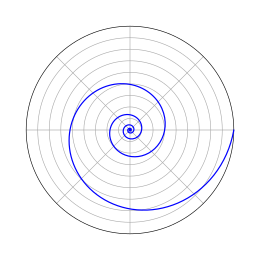
I have been playing around with distance field rendering, inspired by some of Iñigo Quílez's work. Along the way I needed to define analytic distance functions for a number of fairly esoteric geometric primitives, among them the logarithmic spiral:

The distance function for this spiral is not particularly hard to derive, but the derivation isn't entirely straightforward, and it isn't documented anywhere else, so I thought I would share. I am only going to deal with logarithmic spirals centered on the origin, but the code is trivial to extend for spirals under translation.

Spirals are considerably more tractable in polar coordinates, so we start with the polar coordinate form of the logarithmic spiral equation:

\( r = ae^{b\Theta} \) (1)

Where (roughly) a controls the starting angle, and b controls how tightly the spiral is wound.

Since we are given an input point in x,y Cartesian form, we need to convert that to polar coordinates as well:

\( r_{target} = \sqrt{x^2 + y^2},; \Theta_{target} = atan(y/x) \)

Now, we can observe that the closest point on the spiral to our input point must be on the line running through our input point and the origin - draw the line on the graph above if you want to check for yourself. Since the logarithmic spiral passes through the same radius line every 360°, this means than the closest point must be at an angle of:

\( \Theta_{final} = \Theta_{target} + n *360^{\circ} \) (2)

Where n is a non-negative integer. We can combine (1) and (2), to arrive at an equation for r in terms of n:

\( r = ae^{b(\Theta_{target} + n*360^{\circ})} \) (3)

Which means we can find r if we know n. Unfortunately we don't know n, but we do know rtarget, which is an approximation for the value of r. We start by rearranging equation (3) in terms of n:

\( n = \frac{\frac{ln(\frac{r}{a})}{b} - \Theta_{target}}{360^{\circ}} \) (4)

Now, feeding in the value of rtarget for r will give us an approximate value for n. This approximation will be a real (float, if you prefer), and we can observe from the graph above that the closest point must be at either the next larger or smaller integer value of n.

If we take the floor and ceil of our approximation for n, we will have both integer quantities, and can feed each value back into equation (3) to determine the two possible values of r, r1 and r2. The final step involves finding which of these is the closest, and the distance thereof:

\( min(|r_1-r|, |r_2-r|) \)

And there you have it:

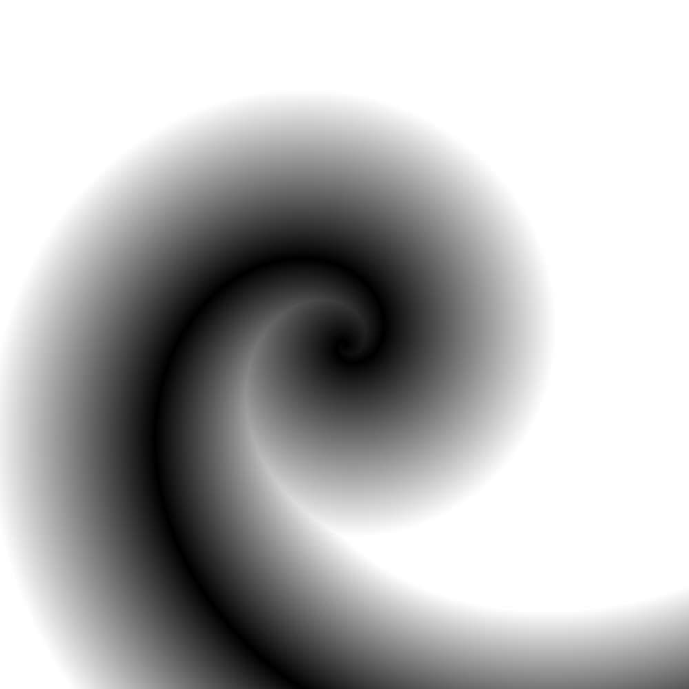
The python source code below produces the image shown above, as a 1000x1000 pixel image PNM image written to stdout. If you aren't familiar with the PNM format, it is an exceedingly simple ascii-based analogue of a bitmap image, and can be loaded directly in GIMP.

import math

def spiral(x, y, a=1.0, b=1.0):
  # calculate the target radius and theta
  r = math.sqrt(x*x + y*y)
  t = math.atan2(y, x)

  # early exit if the point requested is the origin itself
  # to avoid taking the logarithm of zero in the next step
  if (r == 0):
    return 0

  # calculate the floating point approximation for n
  n = (math.log(r/a)/b - t)/(2.0*math.pi)

  # find the two possible radii for the closest point
  upper_r = a * math.pow(math.e, b * (t + 2.0*math.pi*math.ceil(n)))
  lower_r = a * math.pow(math.e, b * (t + 2.0*math.pi*math.floor(n)))

  # return the minimum distance to the target point
  return min(abs(upper_r - r), abs(r - lower_r))

# produce a PNM image of the result
if __name__ == '__main__':
  print 'P2'
  print '# distance field image for spiral'
  print '1000 1000'
  print '255'
  for i in range(-500, 500):
    for j in range(-500, 500):
      print '%3d' % min( 255, int(spiral(i, j, 1.0, 0.5)) ),
    print